If you haven’t already, please check out my primer on binary classification in supervised learning. I’ll continue where we left off in the context of a recurrent neural network.
Recall that Recurrent Neural Networks (RNNs) are a class of neural networks designed to handle sequential data, as its connections form directed cycles. This really means that we have some sort of memory, where we consider both the current and previous states in our objective function for each neuron. We refer to these dependencies as hidden states. Today we’ll start with the simple formulation of an RNN using the Backpropagation Through Time (BPTT) algorithm and then establish longer temporal connections through specialized neurons like GRUs or LSTMs. We’ll use each of these architectures to recover a noisy signal.
Let’s examine this mathematically, where:
Input vector: \( x_t \)
Dimensionality of hidden state: \( h_t \)
Output vector: \( y_t \)
Weight matrix for input to hidden layer transition: \( W_{xh} \)
Weight matrix for hidden layer to hidden layer transition: \( W_{hh} \)
Weight matrix for hidden layer to output transition: \( W_{hy} \)
Hidden layer bias: \( b_h \)
Output bias: \( b_y \)
Hidden state updated by previous states: \( h_t \)
Where \( h_t = f(W_{hh} h_{t-1} + W_{xh} x_t + b_h) \), and \( y_t = g(W_{hy} h_t + b_y) \), with \( f \) being an activation function like \( \tanh \) or \( \text{ReLU} \) and \( g \) for regression or classification.
The initialized hidden state, \( h_0 \), can either be set to all zeros or a learned parameter. Note how \( h_t \) takes into account the last state recursively, which means backpropagation involves multiplying many partials which may lead the gradient to vanish. In RNNs, we use the Backpropagation Through Time (BPTT) algorithm.
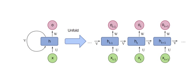
The figure above shows the first part of the BPTT algorithm: unfolding. Here, we convert the cyclic graph into an acyclic graph by expanding the hidden state into its prior dependencies. From here, we compute a forward pass and compute the total loss. After, we compute our backwards pass and compute the gradient of the loss function with respect to each of our parameters. As we did with supervised learning, we adjust our weights to follow the minimization of loss with respect to our parameters, starting from \( t = 0 \) to \( t = T \).
In other words,
\[ W = W - \eta \frac{\partial L}{\partial W} \]
Let’s implement this basic RNN using a MATLAB Script:
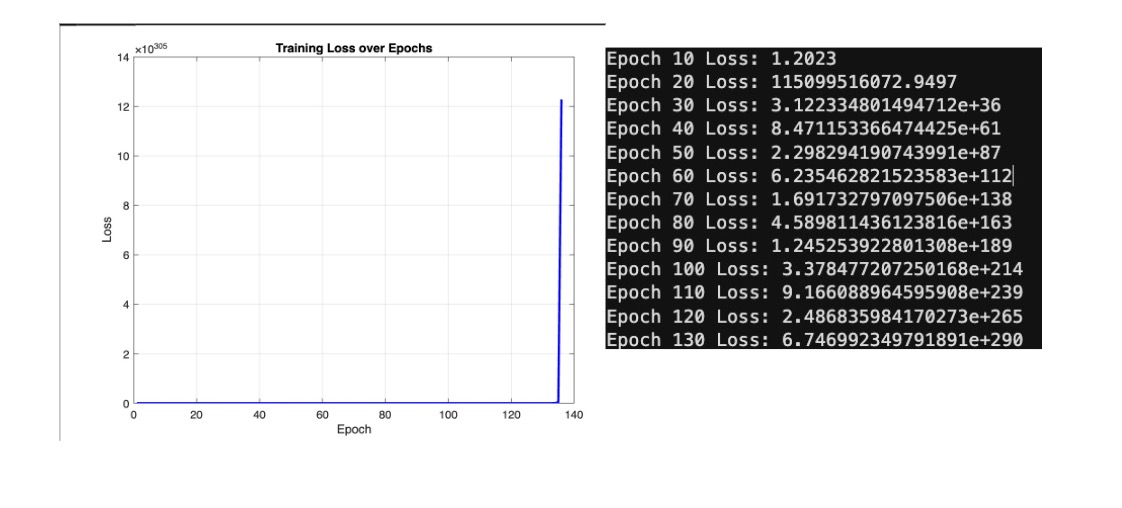
That’s not very good. We’re experiencing an exploding gradient. Since the depth of our network is fairly substantial, our gradients accumulate exponentially. To promote stability, we can induce gradient clipping to limit the gradient from passing 1. We also decrease our learning rate and initialize our weights as smaller values. Let’s see what this does:
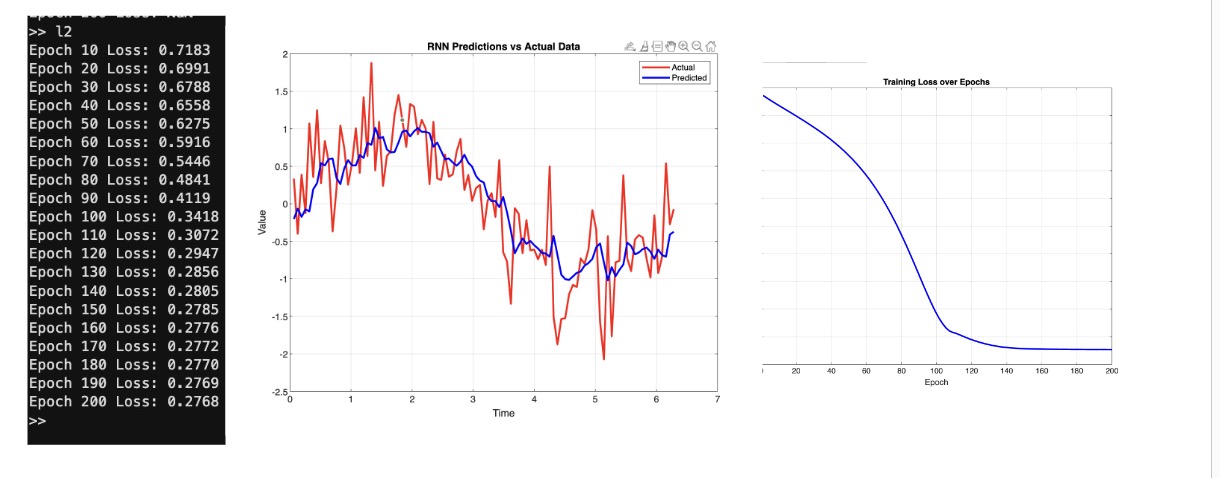
Woah! That’s so much better.
RNNs have difficulty creating long term dependencies because they are bound to care less about earlier input vectors due to the nature of their updated state. Additionally, RNNs still struggle with the vanishing gradient problem due to the potential multiplication of small partial derivatives with respect to the loss surface. For this, we have a few methods: attention scores, LSTMs, GRUs, and regularization methods. We’ve already talked about the latter, and due to the recency of attention scores, we begin with a discussion of LSTMs and GRUs.
Gated Recurrent Units (GRUs)
The Gated Recurrent Unit (GRU) uses an update gate, reset gate, and current memory content to handle the vanishing gradient problem and capture long-term dependencies. We use GRUs when model size and training speed are vital or when there is a smaller range of temporal dependencies.
- Update gate weight matrix: \( W_z \)
- Reset gate weight matrix: \( W_r \)
- Candidate hidden state weight matrix: \( W \)
- Previous hidden state: \( h_{t-1} \)
- Update gate bias: \( b_z \)
- Reset gate bias: \( b_r \)
- Candidate hidden state bias: \( b_h \)
The update gate of a GRU decides how much of the past information needs to be passed to the future. Here is the sigmoid function.
\[ z_t = \sigma(W_z [h_{t-1}, x_t] + b_z) \]
The reset gate decides how much of past information to forget.
\[ r_t = \sigma(W_r [h_{t-1}, x_t] + b_r) \]
The current memory content utilizes the reset gate to determine how important past information is. It generates a candidate activation state, \( \tilde{h} \), given the previous state and forget gate, and linearly interpolates a new hidden state between that candidate state and the previous state. Here, the update gate controls the extent of mixing.
\[ \tilde{h} = \tanh(W [x_t, r_t \odot h_{t-1}] + b_h) \]
\[ h_t = (1 - z_t) \odot \tilde{h} + z_t \odot h_{t-1} \]
Our output vector is just:
\[ y_t = f(W_y h_t + b_y) \]
Similarly to our weight matrices in RNNs, we use backpropagation and an optimizer to find our optimal weights and biases by computing the derivative of the loss function with respect to the parameter surface. Let’s modify our current set up so we use a GRU to capture longer term dependencies and prevent a vanishing gradient. Due to the nature of GRUs, we’ll also decrease the learning rate, increase the number of hidden units, and refine our weight initialization. Let’s also improve the fidelity of our data by using a time step of 1000 instead of 100.
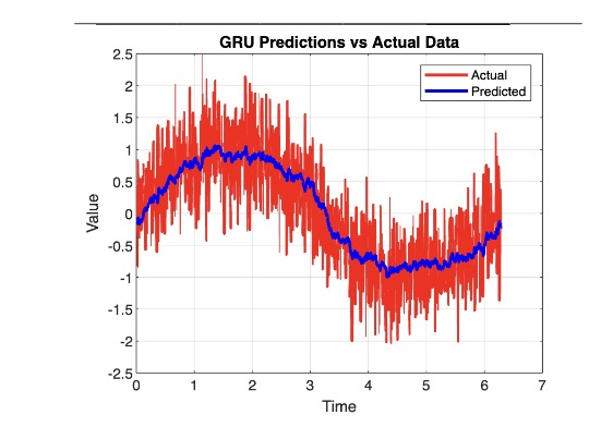
At this stage, we’re more interested in how our predicted values match the original generated wave without noise. Let’s compare our RNN model to our GRU model in terms of signal recovery:
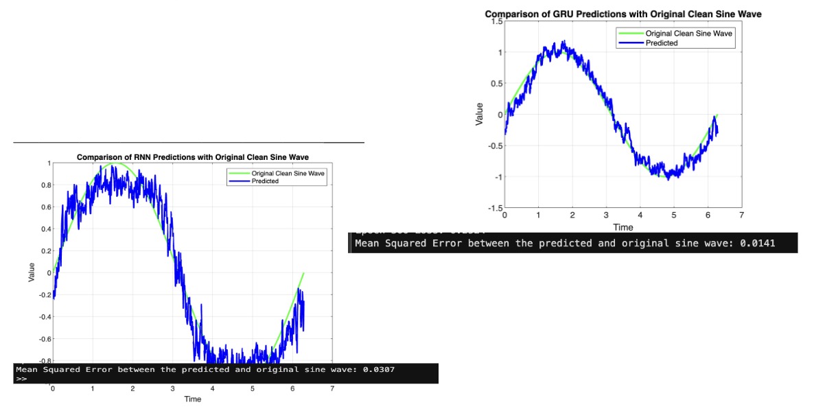
In this case, the GRU does a better job recovering the original signal amidst noise. Let’s move on to our discussion of LSTMs, which are close relatives to the GRU.
Long Short-Term Memory (LSTM) Networks
Long Short-Term Memory (LSTM) networks have three gates (input, forget, and output), and handle the vanishing gradient problems of standard RNNs. LSTM maintains both the cell state and the hidden state \( c_t \) and \( h_t \).
- Forget gate weight matrix: \( W_f \)
- Input gate weight matrix: \( W_i \)
- Candidate memory cell weight matrix: \( W_c \)
- Output gate weight matrix: \( W_o \)
- Previous hidden state: \( h_{t-1} \)
- Forget gate bias: \( b_f \)
- Input gate bias: \( b_i \)
- Candidate memory cell bias: \( b_c \)
- Output gate bias: \( b_o \)
The input gate decides what to update in the cell state.
\[ i_t = \sigma(W_i [h_{t-1}, x_t] + b_i) \]
The forget gate decides what to discard from the cell state.
\[ f_t = \sigma(W_f [h_{t-1}, x_t] + b_f) \]
The candidate memory cell updates the cell state.
\[ \tilde{c} = \tanh(W_c [h_{t-1}, x_t] + b_c) \]
The cell state is a combination of the input gate, candidate memory cell, forget gate, and previous cell state.
\[ c_t = f_t \odot c_{t-1} + i_t \odot \tilde{c} \]
The output gate decides which part of the cell state to output.
\[ o_t = \sigma(W_o [h_{t-1}, x_t] + b_o) \]
And we obtain the hidden state from the cell state.
\[ h_t = o_t \odot \tanh(c_t) \]
Our output vector is again just:
\[ y_t = f(W_y h_t + b_y) \]
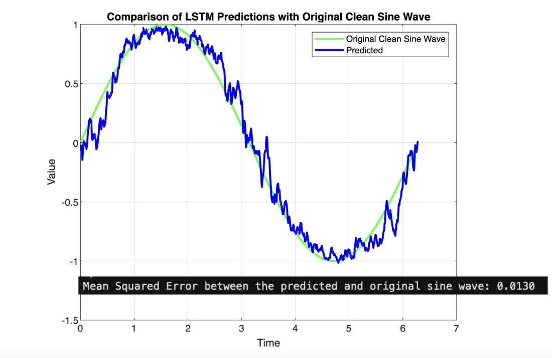
Let’s implement the LSTM architecture into our code. We see a slight improvement over the GRU, but honestly not that noticeable in this case:
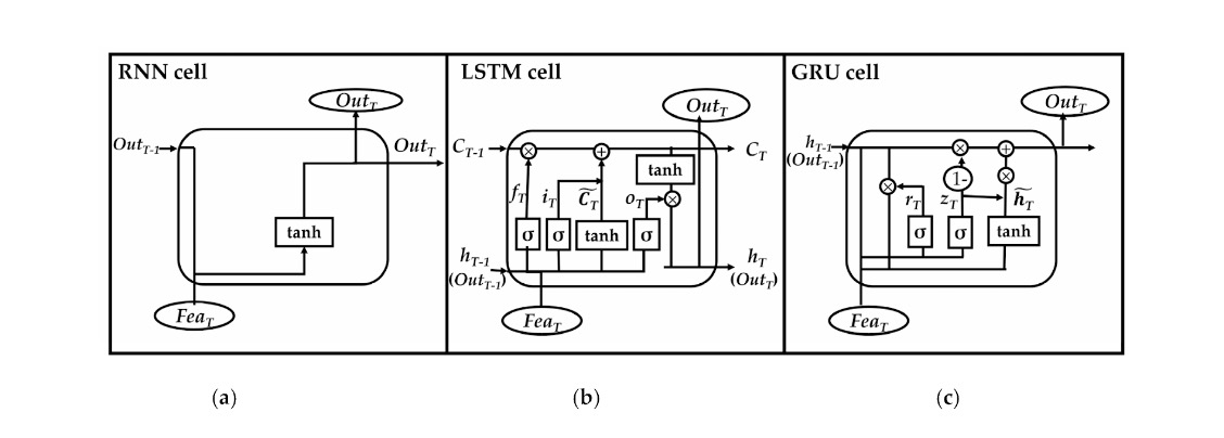
I’ll leave this figure below. It might look a bit frightening at first, but realize that \( f_T \) is the forget gate, \( i_T \) is the input gate, \( C_T \) is the cell state, \( o_T \) is the output gate, \( h_T \) is the hidden state, \( r_T \) is the reset gate, \( z_T \) is the forget gate, \( h_T \) is the candidate state, \( Fea_T \) is a feature vector, and \( Out_T \) is the output.
For MATLAB code, please reach out: